How to Draw Lines on Image and Measure Theor Distance

We have now reached the final installment in our three part series on measuring the size of objects in an image and computing the distance between objects.

Two weeks ago, we started this round of tutorials by learning how to (correctly) order coordinates in a clockwise manner using Python and OpenCV. Then, last week, we discussed how to measure the size of objects in an image using a reference object.

This reference object should have two important properties, including:

1. We know the dimensions (in terms of inches, millimeters, etc.) of the object.
2. It can be easily identifiable in our image (based on either location or appearances).

Given such a reference object, we can use it compute the size of objects in our image.

Today, we are going to combine the techniques used in the previous blog posts in this series and use these methods to compute the distance between objects.

Keep reading to find out how…

Looking for the source code to this post?

Jump Right To The Downloads Section

Measuring distance between objects in an image with OpenCV

Computing the distance between objects is very similar to computing the size of objects in an image — it all starts with the reference object.

As detailed in our previous blog post, our reference object should have two important properties:

• Property #1: We know the dimensions of the object in some measurable unit (such as inches, millimeters, etc.).
• Property #2: We can easily find and identify the reference object in our image.

Just as we did last week, we'll be using a US quarter as our reference object which has a width of 0.955 inches (satisfying Property #1).

We'll also ensure that our quarter is always the left-most object in our image, thereby satisfying Property #2:

Figure 1: We'll identify our reference object based on location, hence we'll always ensure our quarter is the left-most object in the image.

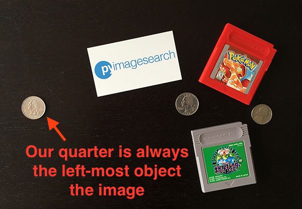
Our goal in this image is to (1) find the quarter and then (2) use the dimensions of the quarter to measure the distance between the quarter and all other objects.

Defining our reference object and computing distances

Let's go ahead and get this example started. Open up a new file, name it distance_between.py , and insert the following code:

# import the necessary packages from scipy.spatial import distance as dist from imutils import perspective from imutils import contours import numpy as np import argparse import imutils import cv2  def midpoint(ptA, ptB): 	return ((ptA[0] + ptB[0]) * 0.5, (ptA[1] + ptB[1]) * 0.5)  # construct the argument parse and parse the arguments ap = argparse.ArgumentParser() ap.add_argument("-i", "--image", required=True, 	help="path to the input image") ap.add_argument("-w", "--width", type=float, required=True, 	help="width of the left-most object in the image (in inches)") args = vars(ap.parse_args())          

Our code here is near identical to last week. We start by importing our required Python packages on Lines 2-8. If you don't already have the imutils package installed, stop now to install it:

$ pip install imutils          

Otherwise, you should upgrade to the latest version (0.3.6 at the time of this writing) so you have the updated order_points function:

$ pip install --upgrade imutils          

Lines 14-19 parse our command line arguments. We need two switches here: --image , which is the path to the input image containing the objects we want to measure, and --width , the width (in inches) of our reference object.

Next, we need to preprocess our image:

# load the image, convert it to grayscale, and blur it slightly image = cv2.imread(args["image"]) gray = cv2.cvtColor(image, cv2.COLOR_BGR2GRAY) gray = cv2.GaussianBlur(gray, (7, 7), 0)  # perform edge detection, then perform a dilation + erosion to # close gaps in between object edges edged = cv2.Canny(gray, 50, 100) edged = cv2.dilate(edged, None, iterations=1) edged = cv2.erode(edged, None, iterations=1)  # find contours in the edge map cnts = cv2.findContours(edged.copy(), cv2.RETR_EXTERNAL, 	cv2.CHAIN_APPROX_SIMPLE) cnts = imutils.grab_contours(cnts)  # sort the contours from left-to-right and, then initialize the # distance colors and reference object (cnts, _) = contours.sort_contours(cnts) colors = ((0, 0, 255), (240, 0, 159), (0, 165, 255), (255, 255, 0), 	(255, 0, 255)) refObj = None          

Lines 22-24 load our image from disk, convert it to grayscale, and then blur it using a Gaussian filter with a 7 x 7 kernel.

Once our image has been blurred, we apply the Canny edge detector to detect edges in the image — a dilation + erosion is then performed to close any gaps in the edge map (Lines 28-30).

A call to cv2.findContours detects the outlines of the objects in the edge map (Lines 33-35) while Line 39 sorts our contours from left-to-right. Since we know that our US quarter (i.e., the reference object) will always be the left-most object in the image, sorting the contours from left-to-right ensures that the contour corresponding to the reference object will always be the first entry in the cnts list.

We then initialize a list of colors used to draw the distances along with the refObj variable, which will store our bounding box, centroid, and pixels-per-metric value of the reference object.

# loop over the contours individually for c in cnts: 	# if the contour is not sufficiently large, ignore it 	if cv2.contourArea(c) < 100: 		continue  	# compute the rotated bounding box of the contour 	box = cv2.minAreaRect(c) 	box = cv2.cv.BoxPoints(box) if imutils.is_cv2() else cv2.boxPoints(box) 	box = np.array(box, dtype="int")  	# order the points in the contour such that they appear 	# in top-left, top-right, bottom-right, and bottom-left 	# order, then draw the outline of the rotated bounding 	# box 	box = perspective.order_points(box)  	# compute the center of the bounding box 	cX = np.average(box[:, 0]) 	cY = np.average(box[:, 1])          

On Line 45 we start looping over each of the contours in the cnts list. If the contour is not sufficiently large (Lines 47 and 48), we ignore it.

Otherwise, Lines 51-53 compute the rotated bounding box of the current object (using cv2.cv.BoxPoints for OpenCV 2.4 and cv2.boxPoints for OpenCV 3).

A call to order_points on Line 59 rearranges the bounding box (x, y)-coordinates in top-left, top-right, bottom-right, and bottom-left order, which as we'll see, is important when we go to compute the distance between object corners.

Lines 62 and 63 compute the center (x, y)-coordinates of the rotated bounding box by taking the average of the bounding box in both the x and y direction.

The next step is to calibrate our refObj :

            # if this is the first contour we are examining (i.e., 	# the left-most contour), we presume this is the 	# reference object 	if refObj is None: 		# unpack the ordered bounding box, then compute the 		# midpoint between the top-left and top-right points, 		# followed by the midpoint between the top-right and 		# bottom-right 		(tl, tr, br, bl) = box 		(tlblX, tlblY) = midpoint(tl, bl) 		(trbrX, trbrY) = midpoint(tr, br)  		# compute the Euclidean distance between the midpoints, 		# then construct the reference object 		D = dist.euclidean((tlblX, tlblY), (trbrX, trbrY)) 		refObj = (box, (cX, cY), D / args["width"]) 		continue          

If our refObj is None (Line 68), then we need to initialize it.

We start by unpacking the (ordered) rotated bounding box coordinates and computing the midpoint between the top-left and bottom-left along with top-right and bottom-right points, respectively (Lines 73-75).

From there, we compute the Euclidean distance between the points, giving us our "pixels-per-metric", allowing us to determine how many pixels fit into --width inches.

Note: See last week's post for a more detailed discussion of the "pixels-per-metric" variable.

Finally, we instantiate our refObj as a 3-tuple consisting of:

1. The sorted coordinates corresponding to the rotated bounding box reference object.
2. The centroid of the reference object.
3. The pixels-per-metric ratio that we'll be using to determine the distance between objects.

Our next code block handles drawing the contours around our reference object and the object we are currently examining, followed by constructing refCoords and objCoords such that (1) the bounding box coordinates and (2) the (x, y)-coordinates of the of the centroid are included in the same arrays:

            # draw the contours on the image 	orig = image.copy() 	cv2.drawContours(orig, [box.astype("int")], -1, (0, 255, 0), 2) 	cv2.drawContours(orig, [refObj[0].astype("int")], -1, (0, 255, 0), 2)  	# stack the reference coordinates and the object coordinates 	# to include the object center 	refCoords = np.vstack([refObj[0], refObj[1]]) 	objCoords = np.vstack([box, (cX, cY)])          

We are now ready to compute the distance between the respective corners and centroids of objects in our image:

            # loop over the original points 	for ((xA, yA), (xB, yB), color) in zip(refCoords, objCoords, colors): 		# draw circles corresponding to the current points and 		# connect them with a line 		cv2.circle(orig, (int(xA), int(yA)), 5, color, -1) 		cv2.circle(orig, (int(xB), int(yB)), 5, color, -1) 		cv2.line(orig, (int(xA), int(yA)), (int(xB), int(yB)), 			color, 2)  		# compute the Euclidean distance between the coordinates, 		# and then convert the distance in pixels to distance in 		# units 		D = dist.euclidean((xA, yA), (xB, yB)) / refObj[2] 		(mX, mY) = midpoint((xA, yA), (xB, yB)) 		cv2.putText(orig, "{:.1f}in".format(D), (int(mX), int(mY - 10)), 			cv2.FONT_HERSHEY_SIMPLEX, 0.55, color, 2)  		# show the output image 		cv2.imshow("Image", orig) 		cv2.waitKey(0)          

On Line 94 we start looping over pairs of (x, y)-coordinates that correspond to our reference object and object of interest.

We then draw a circle representing the (x, y)-coordinates of the current points we are computing the distance between and draw a line to connect the points (Lines 97-110).

From there, Line 105 computes the Euclidean distance between the reference location and the object location, followed by dividing the distance by the "pixels-per-metric", giving us the final distance in inches between the two objects. The computed distance is then drawn on our image (Lines 106-108).

Note: This distance computation is performed for each of the top-left, top-right, bottom-right, bottom-left, and centroid coordinates for a total of five distance comparisons.

Finally, Lines 111 and 112 display the output image to our screen.

Distance measurement results

To give our distance measurement script a try, download the source code and corresponding images to this post using the "Downloads" form at the bottom of this tutorial. Unarchive the .zip file, change directory to the distance_between.py script, and then execute the following command:

$ python distance_between.py --image images/example_01.png --width 0.955          

Below follows a GIF animation demonstrating the output of our script:

Figure 2: Computing the distance between objects in an image with OpenCV.

In each of these cases, our script matches the top-left (red), top-right (purple), bottom-right (orange), bottom-left (teal), and centroid (pink) coordinates, followed by computing the distance (in inches) between the reference object and the current object.

Notice how the two quarters in the image are perfectly parallel to each other, implying that the distance between all five control points is 6.1 inches.

Below follows a second example, this time computing the distance between our reference object and a set of pills:

$ python distance_between.py --image images/example_02.png --width 0.955          

Figure 3: Computing the distance between pills using OpenCV.

This example could be used as input to a pill sorting robot that automatically takes a set of pills and organizes them according to their size and distance from a pill container.

Our last example computes the distance between our reference object (a 3.5in x 2in business card) and a set of 7″ vinyl records and an envelope:

$ python distance_between.py --image images/example_03.png --width 3.5          

Figure 4: A final example of computing the distance between objects using OpenCV and computer vision.

As you can see, in each of these cases, we have successfully computed the distance (in actual, measurable units) between objects in an image.

What's next? I recommend PyImageSearch University.

Course information:
30+ total classes • 39h 44m video • Last updated: 12/2021
★★★★★ 4.84 (128 Ratings) • 3,000+ Students Enrolled

I strongly believe that if you had the right teacher you could master computer vision and deep learning.

Do you think learning computer vision and deep learning has to be time-consuming, overwhelming, and complicated? Or has to involve complex mathematics and equations? Or requires a degree in computer science?

That's not the case.

All you need to master computer vision and deep learning is for someone to explain things to you in simple, intuitive terms. And that's exactly what I do. My mission is to change education and how complex Artificial Intelligence topics are taught.

If you're serious about learning computer vision, your next stop should be PyImageSearch University, the most comprehensive computer vision, deep learning, and OpenCV course online today. Here you'll learn how to successfully and confidently apply computer vision to your work, research, and projects. Join me in computer vision mastery.

Inside PyImageSearch University you'll find:

• ✓ 30+ courses on essential computer vision, deep learning, and OpenCV topics
• ✓ 30+ Certificates of Completion
• ✓ 39h 44m on-demand video
• ✓ Brand new courses released every month , ensuring you can keep up with state-of-the-art techniques
• ✓ Pre-configured Jupyter Notebooks in Google Colab
• ✓ Run all code examples in your web browser — works on Windows, macOS, and Linux (no dev environment configuration required!)
• ✓ Access to centralized code repos for all 500+ tutorials on PyImageSearch
• ✓ Easy one-click downloads for code, datasets, pre-trained models, etc.
• ✓ Access on mobile, laptop, desktop, etc.

Click here to join PyImageSearch University

Summary

In the third and final installment in our series on measuring object sizes, we learned how to take two different objects in an image and compute the distance between them inactual measurable units (such as inches, millimeters, etc.).

Just as we found out in last week's post, before we can (1) compute the size of an object or (2) measure the distance between two objects, we first need to compute the "pixels-per-metric" ratio, used to determine how many pixels "fit" into a given unit of measurement.

Once we have this ratio, computing the distance between objects is almost trivially easy.

Anyway, I hope you enjoyed this series of blog posts! If you have any suggestions for a future series, please leave a comment on shoot me a message.

And before you go,be sure to signup for the PyImageSearch Newsletter by entering your email address in the form below!

Download the Source Code and FREE 17-page Resource Guide

Enter your email address below to get a .zip of the code and a FREE 17-page Resource Guide on Computer Vision, OpenCV, and Deep Learning. Inside you'll find my hand-picked tutorials, books, courses, and libraries to help you master CV and DL!

How to Draw Lines on Image and Measure Theor Distance

Source: https://www.pyimagesearch.com/2016/04/04/measuring-distance-between-objects-in-an-image-with-opencv/

Share this post